I will share the concept and applications of “hacker statistics”, an approach for statistical inference. I first try to identify its definition, and then present several examples that apply it. It is considered a quite versitile tool, although there remain a number of questions to study further.
What is hacker statistics? My online search did not bring much information on it, and it looks like there is no established definition. But heavily influenced by Justin Bois’s tutorial[1], I understand it as “simulating data acquisition under an assumption to find the probability of an aspect of interest.” So, next, I will present examples found in Justin Bois’s tutorial[1].
Examples
What is the probability of getting 4 heads when a coin with probability 0.5 of heads is tossed 4 times?
To get an answer to it following the spirit of hacker stats, we do a lot of 4-flip trial recording the number of heads each trial to get an answer, rather than rely on any formula. But, instead of manually doing it, we can realize a lot of coin flipping using a random number generator and for loop. The below code generates 10000 repeats of the 4-flip trial, counting the number of heads. We get the number of trials with 4 heads, and finally the probability of getting 4 heads in 4 tosses.
# Code from [1]

n_all_heads = 0 # Count number of 4-head trials

for n in range(10000): # 10000 repeats of the four flip trials
    heads = np.random.random(size = 4) < 0.5
    n_heads = np.sum(heads)
    if n_heads == 4: # If a given trial has four heads, increase the count
        n_all_heads += 1

n_all_heads / 10000 # What is the probability of getting all four heads?
What is the confidence interval of a sample?
Suppose we have an observed data set of the rainfall amount in millimeters ([122.1, 69.8, 29.6, …, 65.8, 58.2, 130.4]). To get a confidence interval of the mean using hacker stats, we need to be able to simulate repeated measurements, and here comes ‘bootstrapping’, sampling a dataset with replacement.
The below code implements bootstrapping using np.random.choice() in a for loop. It generates 10000 samples, and calculates the mean of each of them. That is, a sampling distribution of the mean is made, and a confidence interval is found by looking at 2.5 and 97.5th percentiles.
bs_replicates = np.empty(10000)

for i in range(10000):

    # Generate a bootstrap sample
    bs_sample = np.random.choice(rainfall, size = len(rainfall)) # Resampling engine
    bs_replicates[i] = np.mean(bs_sample)

# 95 percent confidence interval
conf_int = np.percentile(bs_replicates, [2.5, 97.5])
Is the amount of rainfall in November and June different?
Suppose we have a dataset, a record of the amount of rainfall during November and June. To see if these months have different amount of rainfall indeed, we set the following hypothesis to test:
\[H_0: \mu_{nov} = \mu_{jun}\newline H_1: \mu_{nov} \not = \mu_{jun}\]To do the test with hacker stats, we need to generate many sets of data considering the null hypothesis is true. As a simulation method, there is permutation resampling: merge the two data sets, and iteratively divide the all values into two groups of the same sizes as the two data sets, in every possible way (every possible permutation)[2]. For each iteration, the difference of the two groups’ means is calculated, and we finally check where the observed difference locates in the distribution of these simulated differences.
diff_observed = np.mean(rain_june) - np.mean(rain_november)

perm_replicates = np.empty(10000)

for i in range(10000): # 10000 iterations
    # Generate a permutation sample
    perm_sample_1, perm_sample_2 = permutation_sample(rain_june, rain_november)

    # Compute the test statistic
    perm_replicates[i] = np.mean(perm_sample_1) - np.mean(perm_sample_2)

# Plot the histogram
plt.hist(perm_replicates, density=True)
plt.xlabel('Mean difference')
plt.ylabel('PDF')

# Plot vertical lines at the absolute of the observed difference and negative to it
plt.axvline(np.abs(diff_observed), color = 'r')
plt.axvline(np.abs(diff_observed)*-1, color = 'r')
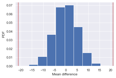
empirical_diff_means = np.mean(rain_november) - np.mean(rain_june)
p = np.sum(perm_replicates >= empirical_diff_means) / len(perm_replicates)
For a p-value, we get the proportion of the distribution where the absolute difference was greater than the absolute value of the observed difference (as the example is the two-tailed test).
We have looked around the examples that apply the hacker stats technique for different questions, and I believe that you got an idea on what hacker stats is.
To the best of my knowledge, there are three methods that realize hacker stats [1][3][5]:
- Use of an existing model
- Permutation sampling
- Bootstrapping
Given them, I wondered about how different results of them would be, when applied to the sample problem. Adapting materials that were found in Bois’ tutorial[1] and Udacity[5], I performed two sample z-test of proportions using each of the three methods.
Two sample z-test of proportions (e.g., A/B testing of click-through rate)
Suppose we have to determine whether the new banner design leads to a better click through rate (CTR) than the old one, and we have the below dataset that tells her group and whether she clicked or not, for each unique user (6328 rows × 2 columns).
| group | clicked | |
|---|---|---|
| 5640 | control | True |
| 376 | control | False |
| 4247 | control | True |
| 2746 | control | False |
| 651 | control | False |
| ... | ... | ... |
| 5157 | experiment | False |
| 4490 | experiment | False |
| 7745 | experiment | True |
| 942 | experiment | False |
| 5255 | experiment | True |
A hypothesis has been made like this:
\[H_0: p_{exp} - p_{ctl} \leq 0\newline H_1: p_{exp} - p_{ctl} > 0\]Permutation sampling
First, I present use of permutation sampling, borrowing code from [1]. The below generates 10000 CTR differences between 10000 resampled pairs of the control and experiment groups.
# ctl_df, a dataframe made by extracting control group records from 'both_df'
# exp_df, experiment group records

ctl_ctr = np.sum(ctl_df['clicked']) / len(ctl_df)
exp_ctr = np.sum(exp_df['clicked']) / len(exp_df)

obs_diff = exp_ctr - ctl_ctr

ctl = ctl_df['clicked'].values
exp = exp_df['clicked'].values

diffs_pm = np.empty(10000)

for i in range(10000):

    # Concatenate the data sets: data
    data = np.concatenate((ctl, exp))

    # Permute the concatenated array: permuted_data
    permuted_data = np.random.permutation(data)

    # Split the permuted array into two: perm_sample_1, perm_sample_2
    ctl_perm_sample = permuted_data[:len(ctl)]
    exp_perm_sample = permuted_data[len(exp):]

    diff_sample = np.sum(exp_perm_sample) / len(exp_perm_sample) - \
                np.sum(ctl_perm_sample) / len(ctl_perm_sample)

    # Compute the test statistic
    diffs_pm[i] = diff_sample

p = np.sum(diffs_pm > obs_diff) / len(diffs_pm)
print('p-value =', p)
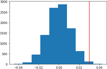
This is the histogram of the CTR differences (test statistics acquired with the resampling), with a line indicating the observed difference (p-value is 0.0027):
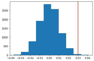
We can get a p-value by dividing the number of differences larger than the observed difference by the total number of values.
p = np.sum(diffs_pm > obs_diff) / len(diffs_pm)
print('p-value =', p)
Bootstrapping
Second, I test the hypothesis by generating samples using the bootstrap method.
# 1) Compute the observed difference
obs_diff = exp_ctr - ctl_ctr

# 2) Simulate the sampling distribution for the difference in proportions
diffs_bt = []
for _ in range(10000):
    # Pick from the whole data with replacement
    b_samp = both_df.sample(both_df.shape[0], replace = True)

    ctl_samp = b_samp.query('group == "control"')
    exp_samp = b_samp.query('group == "experiment"')

    ctl_samp_ctr = ctl_samp['clicked'].sum() / len(ctl_samp)
    exp_samp_ctr = exp_samp['clicked'].sum() / len(exp_samp)

    diffs_bt.append(exp_samp_ctr - ctl_samp_ctr)
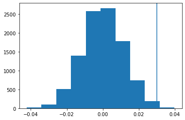
Next, using the above sampling, a distribution under the null hypothesis is simulated, by creating a random normal distribution centered at 0, with the same spread and size.
diffs_arr = np.array(diffs_bt)
null_vals = np.random.normal(0, diffs_arr.std(), diffs_arr.size)
plt.hist(null_vals)
plt.axvline(x = obs_diff);
To get a p-value:
(null_vals > obs_diff).mean()
This is the histogram of the simulated CTR rate differences (p value is 0.0039):
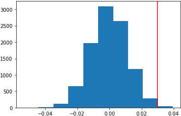
Use of binomial distribution
As shown below, sample acquistion from a binonimal distribution can be simulated using np.random.choice().
# Calculate a click-through-rate under the null hypothesis
p_null = np.sum(both_df['clicked']) / len(both_df)

diffs_bd_1 = []

for _ in range(10000):
    new_page_converted = np.random.choice([1,0], size = n_exp, replace = True, p = (p_null, 1-p_null))
    old_page_converted = np.random.choice([1,0], size = n_ctl, replace = True, p = (p_null, 1-p_null))

    diffs_bd_1.append(new_page_converted.mean() - old_page_converted.mean())
This is the histogram of the results (p value is 0.0049):
Or, np.random.binomial() can be used as below.
new_simulation = np.random.binomial(n_exp, p_null, 10000)/n_exp
old_simulation = np.random.binomial(n_ctl, p_null, 10000)/n_ctl
diffs_bd_2 = new_simulation - old_simulation
This is the histogram of the results (p value is 0.0045):
In addition to the use of hacker stats, I calculated a p-value using the parametric method (statsmodels.stats.proportion.proportions_ztest()).
from statsmodels.stats.proportion import proportions_ztest, proportion_confint

successes = [928, 932]
nobs = [n_exp, n_ctl]

z_stat, pval = proportions_ztest(successes, nobs=nobs, alternative = 'larger')
(lower_con, lower_treat), (upper_con, upper_treat) = proportion_confint(successes, nobs=nobs, alpha=0.05)

print(f'z statistic: {z_stat:.2f}')
print(f'p-value: {pval:.5f}')
z statistic: 2.62
p-value: 0.00442
You can find all the code in my Github page.
Let’s compare all the p-values:
- Permutation method: 0.0027
- Bootstrapping: 0.0039
- Use of binomial distribution with np.random.choice(): 0.0045
- Use of binomial distribution with np.random.binomial(): 0.0049
And, with the parametric method, 0.00442
Since we generated samples using random number generators, the results with the hackter stats methods are not fixed ones. I ran the code a few times, and compared them as below:
perm 0.0027 < boot 0.0039 < para 0.00442 < bi 0.0045 < choice 0.0049
choice 0.0026 < perm 0.003 < boot 0.0039 < para 0.00442 < bi 0.0054
perm 0.0013 < choice 0.0033 < boot 0.0037 < bi 0.0039 < para 0.00442
perm 0.0025  < para 0.00442 < choice 0.0046 < boot 0.0051 < bi 0.0053
Given the results, the below questions came to my mind:
- The p values are somewhat different each other. Which should we pick as a final result? Which one is the most trustable?
- In my observation, the permutation sampling results in a smaller p-value than the bootstrapping. Will it be always true no matter what data are tested?
References
- Justin Bois. Datacamp. Statistical thinking (1) and Statistical thinking (2)
- Wikipedia. Permutation test
- Yevgeniy (Gene) Mishchenko. Bootstrapping vs. Permutation Testing
- Matthew E. Parker. Resampling (Bootstrapping & Permutation Testing)
- Udacity, Data Analyst Nanodegree
- Jake Vanderplas. Statistics for Hackers - PyCon 2016