Let’s say, you want to identify groups of customers to treat each group with different strategies. If you have a dataset containing features describing customers’ various aspects such as age, occupation, living area, spending behavior and so on, clustering methods can help you figure it out. Hierarchical clustering and KMeans clustering combined with PCA (Principal Component Analysis) are often used in various clustering methods. In this post, I will present how to implement hierarchical clustering, KMeans clustering, and both on PCA features, using SciPy and Scikit-learn libraries in Python.
This description is guided by Asish Biswas’ worked example [1, 2, 3], which aims to show you how to apply the STP (Segmentation, Targeting, Positioning) marketing framework. The dataset used contains demographic information of 2000 customers, as follows:
- Sex – categorical, 0: male, 1: female
- Marital status – categorical, 0: single, 1: non-single
- Age – numerical
- Education – categorical, 0: unknown, 1: high school, 2: university, 3: graduate
- Income – numerical
- Occupation – categorical, 0: unemployed, 1: official, 2: management
- Settlement size – categorical, 0: small city, 1: mid city, 2: big city
I will first talk about initial data exploration and do preprocessing. Then, I will show implementation of the clusterings one by one and then compare results of them. You can find full implementation and code in my github repository.
Data Exploration and Preprocessing
Let’s first look at several rows of the dataset to get familar with it.
| Sex | Marital status | Age | Education | Income | Occupation | Settlement size | |
|---|---|---|---|---|---|---|---|
| ID | |||||||
| 100000001 | 0 | 0 | 67 | 2 | 124670 | 1 | 2 |
| 100000002 | 1 | 1 | 22 | 1 | 150773 | 1 | 2 |
| 100000003 | 0 | 0 | 49 | 1 | 89210 | 0 | 0 |
| 100000004 | 0 | 0 | 45 | 1 | 171565 | 1 | 1 |
| 100000005 | 0 | 0 | 53 | 1 | 149031 | 1 | 1 |
I’ve drawn plots to check distribution of each variable and relationship between pairs of the variables.
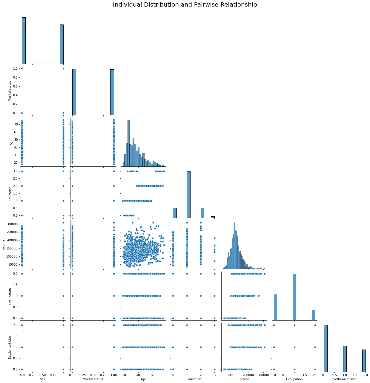
The plots reveal existence of several correlations including relationship between the age and the education and between the occupation and the income.
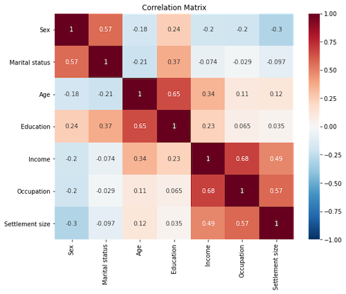
Since distance-based clustering methods are affected by difference of variable scales, I applied standardization to the dataset. I picked the standardization as I will do PCA.
from sklearn import preprocessing
scaler = preprocessing.StandardScaler()
data_sd = scaler.fit_transform(df)
Hierarchical Clustering
I apply euclidean distance for a distance measure and Ward´s linkage for a linkage function.
from scipy.cluster import hierarchy
from scipy.spatial import distance

linkages_sd = hierarchy.linkage(data_sd, method='ward')

plt.figure(figsize = (10, 7))
hierarchy.dendrogram(linkages_sd,
                     show_leaf_counts=False,
                     no_labels=True)
plt.title("Hierarchical Clustering Dendrogram")
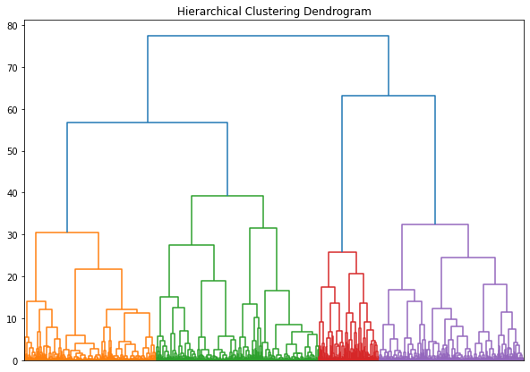
The dendrogram hints that making four groups may be reasonable.
KMeans Clustering
To determine the optimal number of clusters, I draw an elbow plot that tells the degree of variance explained according to the different number of clusters.
from sklearn import cluster

distortions = []
num_clusters = range(1, 11)

for i in num_clusters:
  centroids, labels, inertia = cluster.k_means(data_sd, n_clusters = i, random_state=42)
  distortions.append(inertia)
  labels_list.append(labels)

  elbow_plot = pd.DataFrame({'num_clusters': num_clusters,
                            'distortions': distortions})
  sns.lineplot(x='Number of clusters', y='Sum of squared distances', data = elbow_plot, marker='o')
  plt.xticks(num_clusters)
  plt.title("KMeans Clustering Elbow Graph");
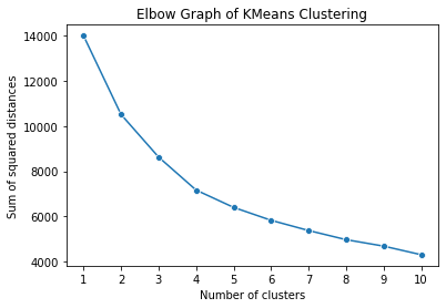
If comparing the magnitude of the slope between two numbers, it tends to remain the same from four. So, it is considered best to make four groups.
PCA
In identifying principal components, let’s first import the sklearn library and create a PCA object with the scaled dataset.
from sklearn import decomposition

pca = decomposition.PCA()
pca.fit(data_sd)
We draw a plot that shows the degree of the explained variance accumulated with additional component.
plt.figure(figsize=(9, 5))
plt.plot(range(1, 8), pca.explained_variance_ratio_.cumsum(), marker='o')
plt.xlabel('Number of components')
plt.ylabel('Cumulative explained aariance')
plt.title("Cumulative Explained Variance by Number of Principal Components");
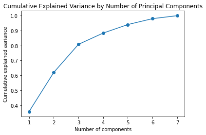
In the above plot, we can see that the first three components explain 80% of the variance, which is considered acceptable [4]. So, I make an instance of the model with three for a number of components and fit it on the dataset. Then, I make a dataframe and heatmap with it to see a loading score of each variable for each component.
pca = decomposition.PCA(n_components=3)
pca.fit(data_sd)

df_pca_components = pd.DataFrame(
    data=pca.components_.round(4),
    columns=df.columns.values,
    index=['component 1', 'component 2', 'component 3'])

s = sns.heatmap(
    df_pca_components,
    vmin=-1,
    vmax=1,
    cmap='RdBu_r',
    annot=True
)
plt.title('Correlation Matrix for Principal Components and Original Features');
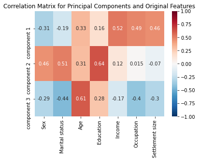
With the above heatmap, we can see that:
- Component 1 has a positive association with Income, Occupation, and Settlement Size
- Component 2 has a positive association with Sex, Martital Status, and Education
- Component 3 has a positive association with Age and a negative association with Martital Status and Occupation.
Hierarchical Clustering and KMeans Clustering on PCA Features
Let’t run a hierarchical clustering model and KMeans on the three principal components.
I first obtain a new dataset by transforming the original scaled dataset on the three principal components and then run a model on it.
pca_scores = pca.transform(data_sd)
linkages_pca = hierarchy.linkage(pca_scores, method='ward')
I do not bring a dendrogram of the result here; you can find it in my github repository. If you see it, you will find that making four groups is a reasonable decision.
I plot the segments with respect to the first two components as below.
labels_hc_pca = hierarchy.fcluster(linkages_pca, t=4, criterion='maxclust')

df_hc_pca = pd.concat([df.reset_index(drop=True), pd.DataFrame(pca_scores)], axis=1)
df_hc_pca.columns.values[-3:] = ['component 1', 'component 2', 'component 3']
df_hc_pca['label'] = labels_hc_pca

plt.figure(figsize=(10, 8))
sns.scatterplot(
    x=df_hc_pca['component 1'],
    y=df_hc_pca['component 2'],
    hue=df_hc_pca['label'],
    palette=['b','m','g','r']
)

plt.title('Hierarchical Clustering on Principle Components');
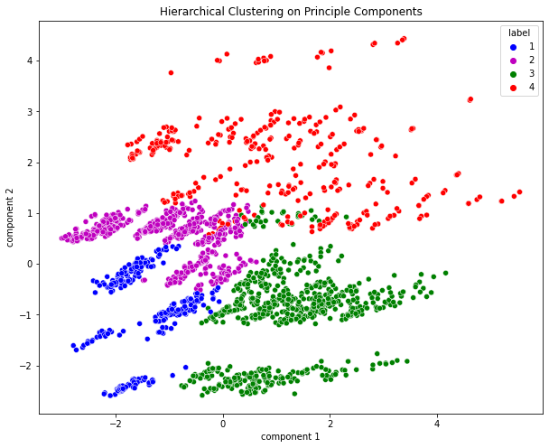
I think the segments are well seperated in overall, although the label 4 overlaps the label 2 and 3 a bit.
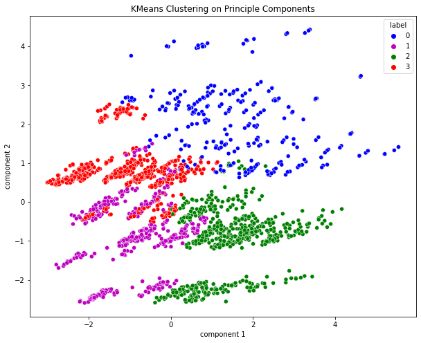
KMeans Clustering on PCA Features
Finally, we run a KMeans clustering model on the three principal components. Based on the elbow graph that you can find in the github repository, I pick four as a number of clusters.
centroids, labels, inertia = cluster.k_means(pca_scores, n_clusters = 4, random_state=42)
Comparison
Now, we have four different versions of segmentation on the dataset. Below is a summary of each version (mean value of each variable for each cluster), in order of hierarchical clustering, KMeans clusteirng, hierarchical clustering with PCA, and KMeans clustering with PCA.
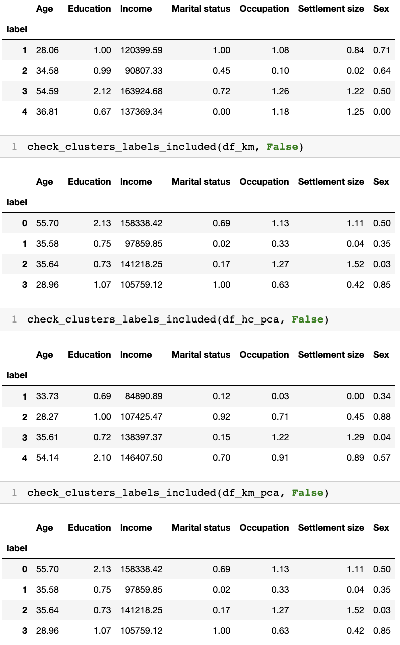
Before getting the above, I’ve printed out a raw result of each version, done some eyeballing, and re-ordered it based on the age and income variable so that:
- Label 1, the youngest and the third level of income
- Label 2, in the middle level in age and the lowest level of income
- Label 3, in the mdidle level in the age and the second level of income
- Label 4, the eldest and the the top level of income
This segmentatation accord with all the four versions; e.g., the youngest group’s income rank is third in all the versions. The mean age values are simiar each other. But the mean income values are fairly much different. As well, we can see discordance between the versions in the other variables.
I am going to do further analysis on the segmentation done with the Kmeans clustering on principal components.
Exploration of Segments
In this section, I will look into the segments created with the Kmeans clustering on principal components to identify characteristics of each of them.
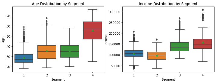
If we compare the median values of the Age, Segment 4 is distinctively high, Segment 2 and 3 are similar, and Segment 1 is the lowest. However, we can see their overlapping with the long whiskers and outliers. The Income plot confirms that Segment 4 is higher than the others, especially Segment 3. However, we can see the wide range of Segment 4 with some extreme outliers on the top and the minimum value lower than Segment 3’s.
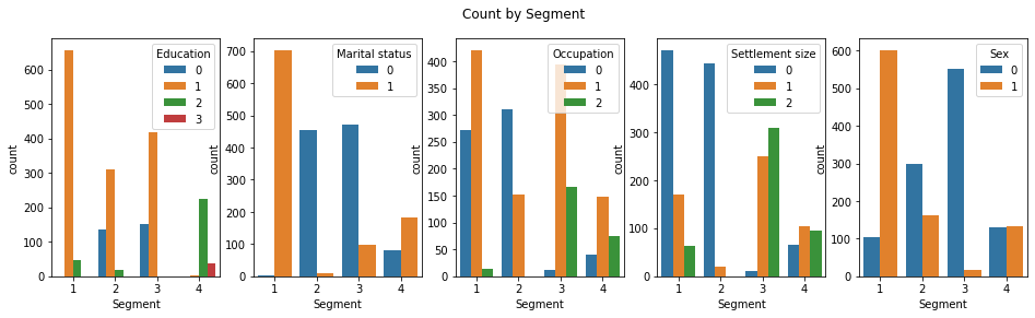
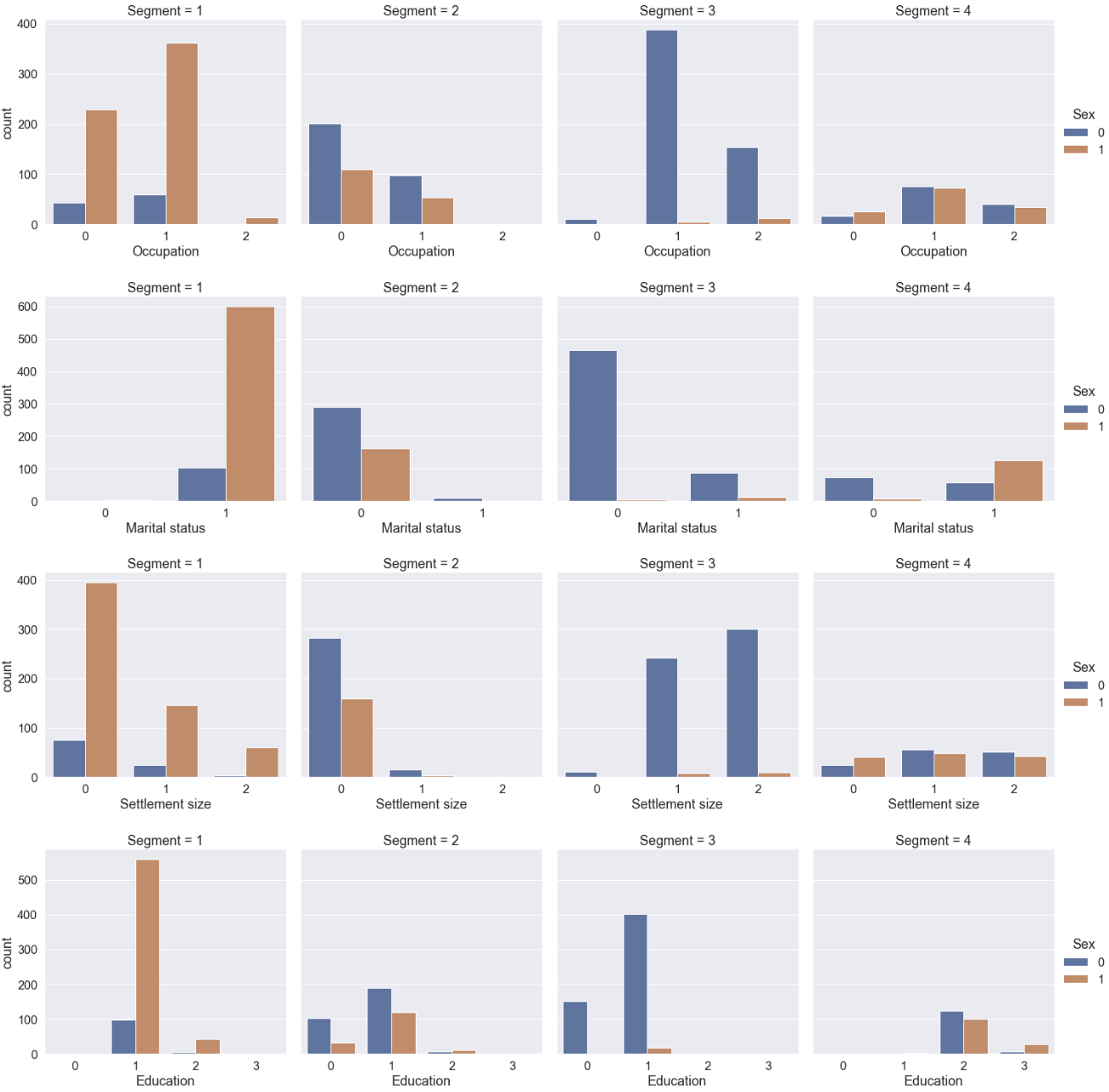
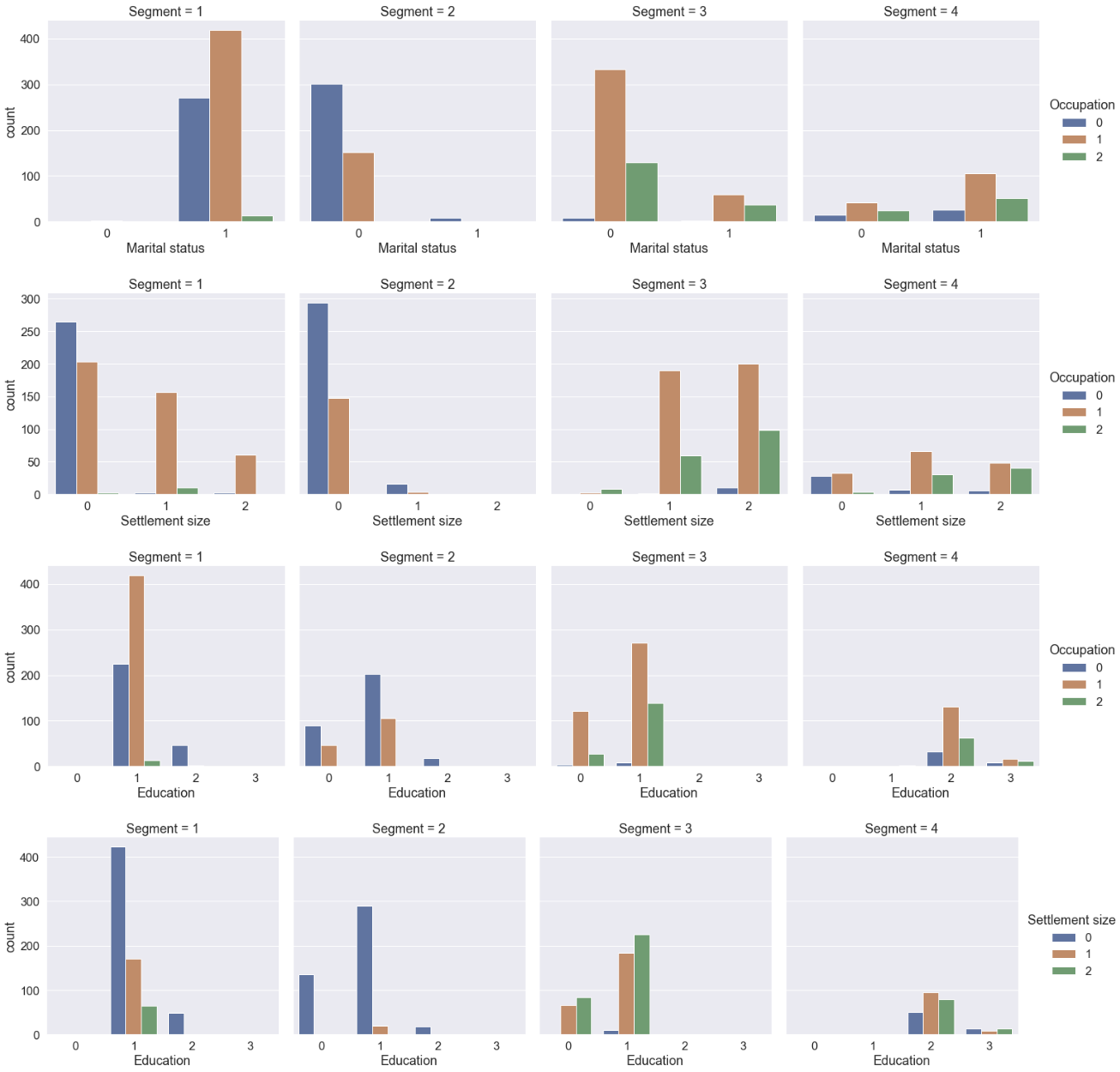
The most distinctive aspect of Segment 1 is that they are mostly high school graduated non-single women in their late 20s. Two-thirds of them live in the small city, half of which have no job. A third live in the mid-sized city with ‘official’ jobs.
Most people of Segment 2 are single living in the small city in the mid 30s. Two-thirds are male and a third, female. Two-thirds are unemployed.
People of Segment 3 are male living the mid or big-sized city with job. The majority is single.
All people of Segment 4 were graduated from university or the higher. Two-thirds are non-single, and a third, single. The sex ratio is one to one. They distributed to all the sizes of the city although more people live in the mid or big-sized city.
Wrapping Up
I have showed how to implement the main clustering methods, hierarchical and KMean clustering combined with PCA. When use the hierarchical clustering, you find out the appropriate number of clusters by looking at a dendrogram. If use the KMean clustering, the elbow graph can help you pick the number of clusters. We have found that the obtained segments are distintive each other, and it suggests usefulness of the clustering methods in segmenting customers.
References
- Asish Biswas. Customer Segmentation with Python (Implementing STP framework - part 1/5)
- Asish Biswas. Customer Segmentation with Python (Implementing STP Framework - Part 2/5
- Asish Biswas. Customer Segmentation with Python (Implementing STP Framework - Part 3/5)
- Elitsa Kaloyanova. What Is Principal Components Analysis?